The output of damid-seq can be found in the results/ directory.

When run with the test data provided in the GitHub repository (.test/reads), the directory structure will be as follows:

results/
├── bam
│   ├── exp1
│   │   ├── Dam.sorted.bam
│   │   ├── Dam.sorted.bam.bai
│   │   ├── Piwi.sorted.bam
│   │   └── Piwi.sorted.bam.bai
│   ├── exp2
│   │   ├── Dam.sorted.bam
│   │   ├── Dam.sorted.bam.bai
│   │   ├── Piwi.sorted.bam
│   │   └── Piwi.sorted.bam.bai
│   └── exp3
│       ├── Dam.sorted.bam
│       ├── Dam.sorted.bam.bai
│       ├── Piwi.sorted.bam
│       └── Piwi.sorted.bam.bai
├── bedgraph
│   ├── exp1
│   │   ├── Piwi-vs-Dam-norm.gatc.bedgraph
│   │   ├── Piwi-vs-Dam.quantile-norm.gatc.bedgraph
│   │   └── Piwi-vs-Dam.rev_log2.bedgraph
│   ├── exp2
│   │   ├── Piwi-vs-Dam-norm.gatc.bedgraph
│   │   ├── Piwi-vs-Dam.quantile-norm.gatc.bedgraph
│   │   └── Piwi-vs-Dam.rev_log2.bedgraph
│   └── exp3
│       ├── Piwi-vs-Dam-norm.gatc.bedgraph
│       ├── Piwi-vs-Dam.quantile-norm.gatc.bedgraph
│       └── Piwi-vs-Dam.rev_log2.bedgraph
├── bigwig
│   ├── average_bw
│   │   └── Piwi.bw
│   ├── bam2bigwig
│   │   ├── exp1
│   │   │   ├── Dam.bw
│   │   │   └── Piwi.bw
│   │   ├── exp2
│   │   │   ├── Dam.bw
│   │   │   └── Piwi.bw
│   │   └── exp3
│   │       ├── Dam.bw
│   │       └── Piwi.bw
│   ├── exp1
│   │   └── Piwi.bw
│   ├── exp2
│   │   └── Piwi.bw
│   └── exp3
│       └── Piwi.bw
├── bigwig_rev_log2
│   ├── average_bw
│   │   └── Piwi.bw
│   ├── exp1
│   │   └── Piwi.bw
│   ├── exp2
│   │   └── Piwi.bw
│   └── exp3
│       └── Piwi.bw
├── deeptools
│   ├── average_bw_matrix.gz
│   ├── correlation.tab
│   ├── heatmap_matrix.gz
│   ├── PCA.tab
│   └── scores_per_bin.npz
├── peaks
│   └── fdr0.01
│       ├── consensus_peaks
│       │   ├── enrichment_analysis
│       │   │   └── Piwi.xlsx
│       │   ├── Piwi.annotated.txt
│       │   ├── Piwi.filtered.bed
│       │   ├── Piwi.geneIDs.txt
│       │   └── Piwi.overlap.bed
│       ├── exp1
│       │   ├── Piwi.bed
│       │   ├── Piwi.data
│       │   ├── Piwi.peaks.gff
│       │   └── Piwi.sorted.bed
│       ├── exp2
│       │   ├── Piwi.bed
│       │   ├── Piwi.data
│       │   ├── Piwi.peaks.gff
│       │   └── Piwi.sorted.bed
│       ├── exp3
│       │   ├── Piwi.bed
│       │   ├── Piwi.data
│       │   ├── Piwi.peaks.gff
│       │   └── Piwi.sorted.bed
│       ├── frip.csv
│       └── read_counts
│           ├── exp1
│           │   ├── Piwi.peak.count
│           │   └── Piwi.total.count
│           ├── exp2
│           │   ├── Piwi.peak.count
│           │   └── Piwi.total.count
│           └── exp3
│               ├── Piwi.peak.count
│               └── Piwi.total.count
├── plots
│   ├── heatmap.pdf
│   ├── mapping_rates.pdf
│   ├── PCA.pdf
│   ├── peaks
│   │   └── fdr0.01
│   │       ├── distance_to_tss.pdf
│   │       ├── enrichment_analysis
│   │       │   └── Piwi
│   │       │       ├── GO_Biological_Process_2018.pdf
│   │       │       ├── GO_Molecular_Function_2018.pdf
│   │       │       └── KEGG_2019.pdf
│   │       ├── feature_distributions.pdf
│   │       └── frip.pdf
│   ├── profile_plot.pdf
│   ├── sample_correlation.pdf
│   └── scree.pdf
├── qc
│   ├── fastqc
│   │   ├── exp1
│   │   │   ├── Dam_fastqc.zip
│   │   │   ├── Dam.html
│   │   │   ├── Piwi_fastqc.zip
│   │   │   └── Piwi.html
│   │   ├── exp2
│   │   │   ├── Dam_fastqc.zip
│   │   │   ├── Dam.html
│   │   │   ├── Piwi_fastqc.zip
│   │   │   └── Piwi.html
│   │   └── exp3
│   │       ├── Dam_fastqc.zip
│   │       ├── Dam.html
│   │       ├── Piwi_fastqc.zip
│   │       └── Piwi.html
│   └── multiqc
│       ├── multiqc_data
│       │   ├── multiqc_citations.txt
│       │   ├── multiqc_data.json
│       │   ├── multiqc_fastqc.txt
│       │   ├── multiqc_general_stats.txt
│       │   ├── multiqc.log
│       │   ├── multiqc_software_versions.txt
│       │   └── multiqc_sources.txt
│       └── multiqc.html
└── trimmed
    ├── exp1
    │   ├── Dam.fastq.gz_trimming_report.txt
    │   └── Piwi.fastq.gz_trimming_report.txt
    ├── exp2
    │   ├── Dam.fastq.gz_trimming_report.txt
    │   └── Piwi.fastq.gz_trimming_report.txt
    └── exp3
        ├── Dam.fastq.gz_trimming_report.txt
        └── Piwi.fastq.gz_trimming_report.txt

50 directories, 118 files

Quality control

FastQC/MultiQC

FastQC is used to do some control check on the trimmed reads.

The output of FastQC is summarized in a MultiQC report (results/qc/multiqc/multiqc.html).

Alignment rates

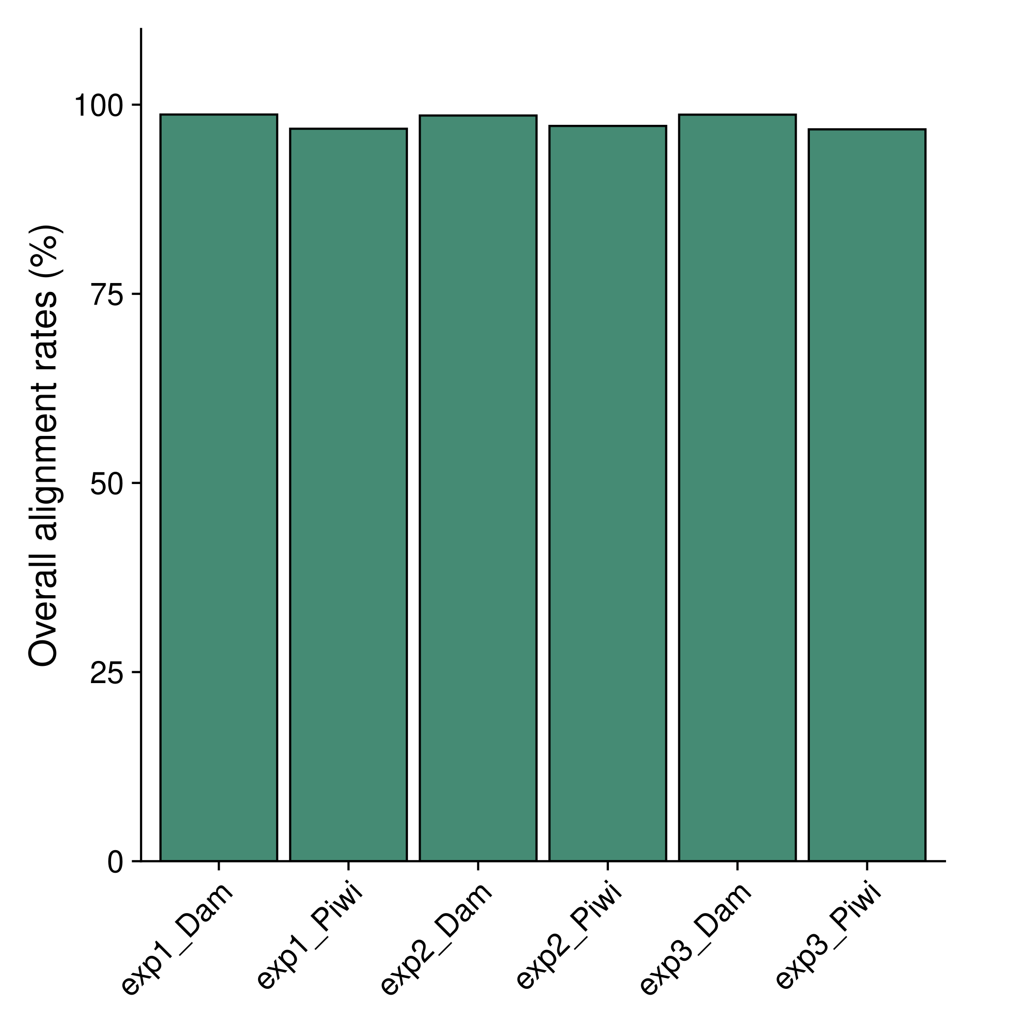
The Bowtie2 alignment rates are summarised in results/plots/mapping_rates.pdf.

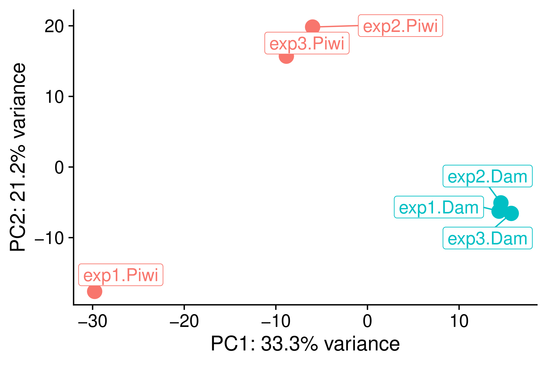
PCA plot of BAM files

A PCA plot of the BAM files is generated to check the consistency of biological replicates. The plot is saved in results/plots/PCA.pdf.

A scree plot is also generated to show the variance explained by each principal component (results/plots/scree.pdf).

Sample correlation heatmap

A correlation (Spearman) heatmap of the BAM files is generated to also check the consistency of biological replicates. The plot is saved in results/plots/sample_correlation.pdf.

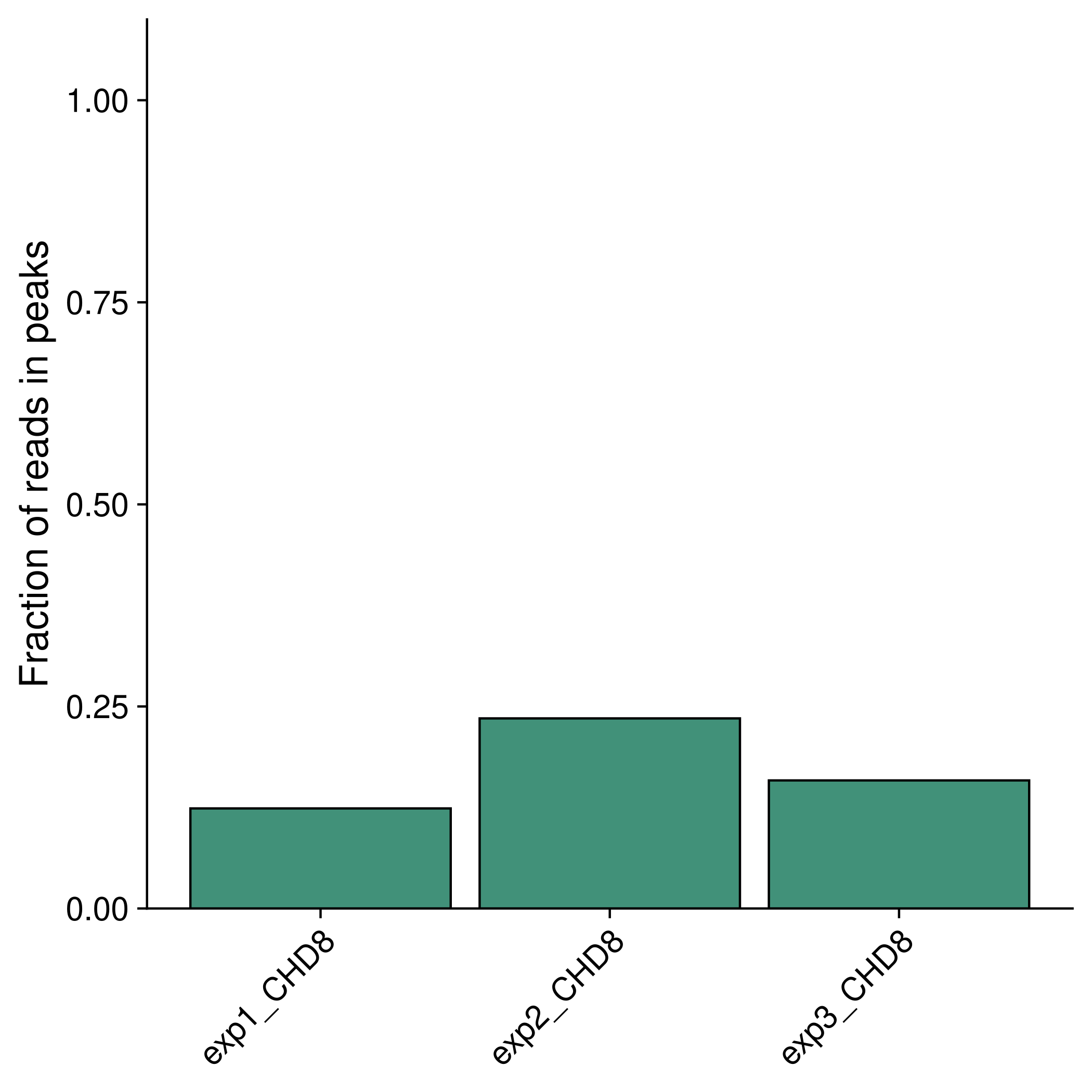
Fraction of reads in peaks (FRiP)

The FRiP is calculated for each sample and plotted in results/plots/peaks/frip.pdf, when using the Perl peak calling script, or results/plots/macs2_[broad or narrow]/fdr[value]/frip.pdf.

Visualization of damid-seq data

Profile plot

Using deepTools, a profile plot is generated to show the average coverage of the reads around defined features of the genome (TSS or gene body). The plot is saved in results/plots/profile_plot.pdf.

Heatmap

A heatmap of the coverage of the reads around defined features of the genome (TSS or gene body) is also generated. The plot is saved in results/plots/heatmap.pdf.

Peak-related plots

Various plot are created relating to peak data.

Distance to TSS

A plot showing the distance of the peaks to the nearest transcription start site (TSS) is generated. The plot is saved in results/plots/[peaks, macs2_broad, macs2_narrow]/fdr[value]/distance_to_tss.pdf.

Binding site distributions

A plot showing the distribution of the peaks across different genomic features is generated. The plot is saved in results/plots/[peaks, macs2_broad, macs2_narrow]/fdr[value]/feature_distributions.pdf.

Differential binding analysis

When the experiment contains more than one non-Dam sample (e.g. HIF1A and HIF2A), DamMapper automatically runs damidBind to identify genomic loci that are differentially bound between conditions. All pairwise comparisons between non-Dam samples are performed.

Note

damidBind requires the Perl peak-calling step to be enabled (peak_calling_perl: run: True) because it uses the resulting GFF peak files alongside the normalized bedgraph profiles.

The analysis is controlled by the following settings in config.yaml:

differential_peaks:
    normalization: quantile # quantile, rpm, scale, none
    fdr: 0.05              # FDR threshold for calling differential peaks
    filter_occupancy: true # Minimum number of samples a locus must have occupancy > 0 in
                           # (true = min replicates, false = no filter, integer = exact number)

Output files are written to results/damidbind/{comparison}/, where {comparison} follows the pattern {sample}_vs_{ref_sample} (e.g. HIF1A_vs_HIF2A):

results/damidbind/
└── HIF1A_vs_HIF2A
    ├── bedgraph/               # symlinks to normalised bedgraph input files
    ├── peaks/                  # symlinks to peak GFF input files
    ├── diagnostic_plots_diff.pdf
    ├── peaks.csv
    ├── venn.pdf
    └── volcano.pdf

diagnostic_plots_diff.pdf

Diagnostic plots produced by damidBind::differential_binding(), showing the distribution of binding scores and model fit across loci.

venn.pdf

Venn diagram showing the overlap between peaks that are gained, lost, or shared between the two compared conditions.

volcano.pdf

Volcano plot of all tested loci, with differentially bound peaks highlighted. Gene labels are cleaned automatically.

peaks.csv

Table of all tested loci with columns for genomic coordinates (chrom, start, end) and the full damidBind statistics (log2 fold-change, p-value, FDR, etc.).